23 Distributions

23.1 Introduction

In the previous chapters, we explored the foundational building blocks of data analysis:

Variables: The fundamental units of data that vary across observations.
Descriptive Statistics: Tools to summarize and describe individual variables, focusing on central tendency, spread, and other key characteristics.

Now, we turn our attention to distributions, which bring these ideas together into a comprehensive view of how data values are spread across their range. A distribution shows not just individual statistics but the entire pattern of variability, helping us answer questions like:

How are values concentrated across the dataset?
Are there patterns of symmetry or asymmetry?
What probabilities are associated with certain ranges of values?

Why Study Distributions?

Understanding distributions is crucial for making sense of data as a whole. While descriptive statistics provide valuable summaries, distributions reveal the underlying structure, enabling us to:

Identify patterns and outliers.
Make informed assumptions for modeling and hypothesis testing.
Visualize how data values relate to one another.

For example, the shape of a distribution tells us whether data is evenly spread, clustered in one region, or skewed to one side. This knowledge helps guide decisions about which analytical tools to apply and what insights to draw.

Connecting the Pieces: From Variables to Distributions

Every variable in a dataset has a distribution that reflects how its values are distributed across observations. Distributions provide a bridge between:

The data itself: Individual observations and variable values.
Descriptive statistics: Measures like mean, standard deviation, skewness, and kurtosis, which characterize the shape and behavior of the distribution.

By studying distributions, we can:

Visualize data holistically.
Use probability to model uncertainties.
Explore relationships between variables more effectively.

In this chapter, you will:

Learn how to visualize distributions using histograms, density plots, and boxplots.
Explore key distribution shapes (e.g., normal, skewed, uniform) and their implications.
Calculate and interpret measures of shape, including skewness and kurtosis.
Understand how distributions inform statistical modeling and hypothesis testing.

This chapter builds on your understanding of variables and descriptive statistics to provide a complete picture of data structure. Distributions are not just summaries—they are the patterns that connect data to decision-making.

23.2 Demonstration Data

We’ll return to the Liberty ships dataset to illustrate distributions. This dataset was first introduced in Section 18.2 and reused in Chapter 21 and Chapter 22 where you can find additional details.

# A tibble: 1,571 × 6
    Unit Yard        Way Direct_Hours Total_Production_Days Total_Cost
   <dbl> <chr>     <dbl>        <dbl>                 <dbl>      <dbl>
 1     1 Bethlehem     1       870870                   244   2615849 
 2     2 Bethlehem     2       831745                   249   2545125 
 3     3 Bethlehem     3       788406                   222   2466811 
 4     4 Bethlehem     4       758934                   233   2414978 
 5     5 Bethlehem     5       735197                   220   2390643 
 6     6 Bethlehem     6       710342                   227   2345051 
 7     8 Bethlehem     8       668785                   217   2254490 
 8     9 Bethlehem     9       675662                   196   2139564.
 9    10 Bethlehem    10       652911                   211   2221499.
10    11 Bethlehem    11       603625                   229   2217642.
# ℹ 1,561 more rows

23.3 What Are Distributions

Imagine arranging all the values of a variable along a line, from the smallest to the largest. Some values will cluster closely together, while others will spread out. This clustering and spreading form the shape of the distribution.

For example, imagine plotting the heights of a group of people. The resulting distribution might have a central peak where most heights cluster (around the average) and taper off on both sides for shorter and taller individuals whose heights are less common.

If the clustering is dense around the average, we say those values are more likely to occur. Conversely, values that are less dense are less likely. This idea of density is central to understanding distributions.

Figure 23.1: The standard Normal distribution illustrated as the density of observation clusters. The smooth curve represents the density of values around the mean (center).

This plot shows individual data points of a random variable \(\mathsf{X}\) that follow a pattern defined by a standard normal distribution. The values of \(\mathsf{X}\) are spread along the x-axis, with the density curve illustrating the theoretical distribution shape that describes where values are most likely to occur. The height of the curve reflects the relative likelihood of values in different regions, with peaks indicating where data points cluster. This pattern is typical of many real-world variables.

23.4 Common Shapes of Distributions

There are hundreds of known probability distributions, each with a different shape. Some common shapes include:

Normal Distribution:
- The bell-shaped curve is symmetrical and centered around the mean.
- Real-world example: Heights of individuals or measurement errors in experiments.
- Entrepreneurial Insight: Normal distributions often serve as a benchmark for modeling and comparison.
Right-Skewed Distribution:
- Most values cluster on the left, with a long tail extending to the right.
- Real-world example: Income levels or customer spending.
- Entrepreneurial Insight: Right-skewed distributions highlight data where a small number of observations have disproportionate impact (e.g., big spenders driving sales).
Bimodal Distribution
- Two peaks indicate distinct groups within the data.
- Real-world example: Customer preferences or seasonal sales.
- Entrepreneurial Insight: Bimodal distributions often reveal multiple populations or market segments requiring tailored strategies.

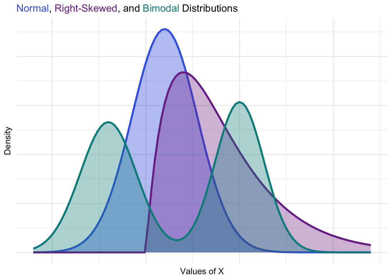
Figure 23.2: The standard normal, right-skewed, and bimodal distributions are some of the many distribution shapes that real-world entrepreneurial data may exhibit

This visualization shows how distributions vary in shape and density. Differences in density imply different actionable insights that the savvy entrerpreneur can leverage to increase success.

23.5 Moments of a Distribution

Moments are a way to describe the shape and behavior of a distribution by summarizing key characteristics. Think of moments as the “landmarks” of a dataset: they tell us where the data is centered, how spread out it is, and whether it has unusual patterns like leaning to one side or having heavy tails. Just as a photograph has features like brightness, contrast, and sharpness, moments capture the features of a distribution’s shape.

First Moment (Central Tendency): Where the data is centered because the values are densely clustered.
Second Moment (Spread): How far values tend to deviate from the center.
Third Moment (Skewness): Whether the data leans left or right.
Fourth Moment (Kurtosis): How much the data is packed into the tails or the peak.

The first moment, central tendency, and the second moment, spread, capture key features of a distribution’s shape. These concepts, already introduced in the descriptive statistics of variables, form the foundation of understanding a distribution. While they provide critical insights, the third and fourth moments—skewness and kurtosis—also reveal important implications for decision-making, especially for entrepreneurs.

Central Tendency: The First Moment

Central tendency represents the predicted value of a variable, often serving as the best guess for its typical value. Among measures of central tendency, the mean is commonly used because it reflects the expected value of a distribution.

Spread: The Second Moment

Variability helps us understand how much individual values differ from the central value. While the mean provides a central point, measures of spread—like variance and standard deviation—help refine decisions based on how widely values deviate from that average.

Below are two normal distributions with the same mean but different levels of variance (spread). Notice how a high-variance distribution is more spread out, indicating a wider range of possible values around the central mean.

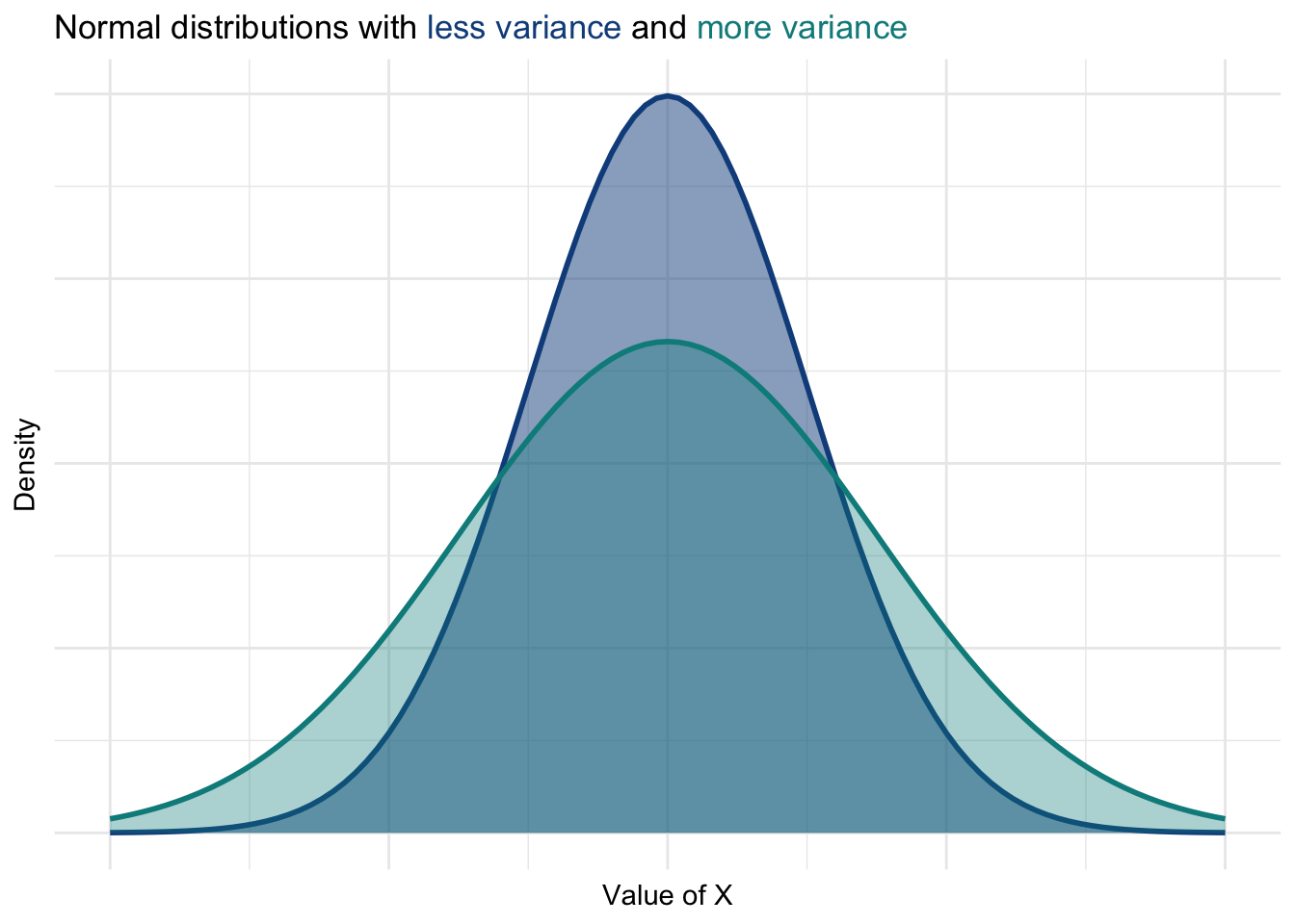
Figure 23.3: Normal distributions with the same mean but different levels of variance

In these plots, you can see that a low-variance distribution clusters more tightly around the mean, whereas a high-variance distribution is more spread out.

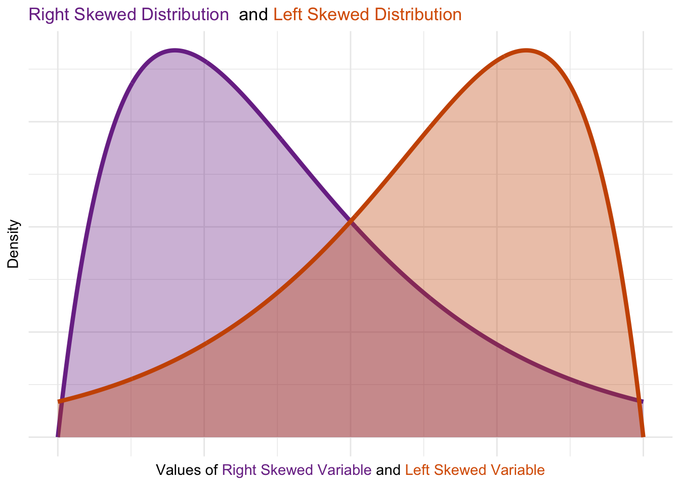
Skewness: The Third Moment

A skewed distribution leans to one side, significantly influencing the interpretation of central tendency. Below are visualizations of positively and negatively skewed distributions:

Right-skewed distributions have values clustered toward the lower end, with a long tail extending to the right.
Left-skewed distributions have values clustered at the higher end, with a long tail extending to the left.

Entrepreneurial Insights from Skewness

Right-Skewed Distributions: A right-skewed distribution might represent income, where most individuals earn below the average, but a few high earners pull the mean higher and stretch the tail. These high earners, if they are also significant spenders, can guide dual marketing strategies:
- Low-end targeting: Capture the majority of customers who spend modestly.
- High-end targeting: Develop premium offerings for the lucrative but smaller high-spending segment.
Left-Skewed Distributions: A left-skewed distribution in product ratings could indicate dissatisfaction from a small but vocal subset of users. This could signal a need for targeted interventions:
- Address key grievances: Identify and resolve issues raised by this subset to improve product perception.
- Mitigate influence risks: If these users significantly influence mainstream customers (e.g., through reviews), proactive trust remediation and tailored compensation may help.
Comparative Analysis of Skewness: In entrepreneurship, comparing the skewness of revenue distributions across regions can reveal disparities in market behavior. For instance, one region might exhibit right skewness (indicating a small base of high-value customers), while another shows a more symmetrical distribution (indicating consistent spending patterns). These insights can inform regional pricing models, promotional campaigns, or product availability strategies.

By understanding and leveraging skewness, entrepreneurs can adapt strategies to cater to both the mainstream and the extremes of their customer base. This ensures that outliers are not ignored but used strategically for growth.

Figure 23.4: Right and left skewed distributions illustrated as changes in the density of data clustering

These visuals highlight how skewness and variance shape a distribution. Skewness reveals asymmetry in value clustering, while variance shows the degree of spread around the central value. Together, these properties inform the choice of central tendency measures and guide decisions on interpreting data patterns.

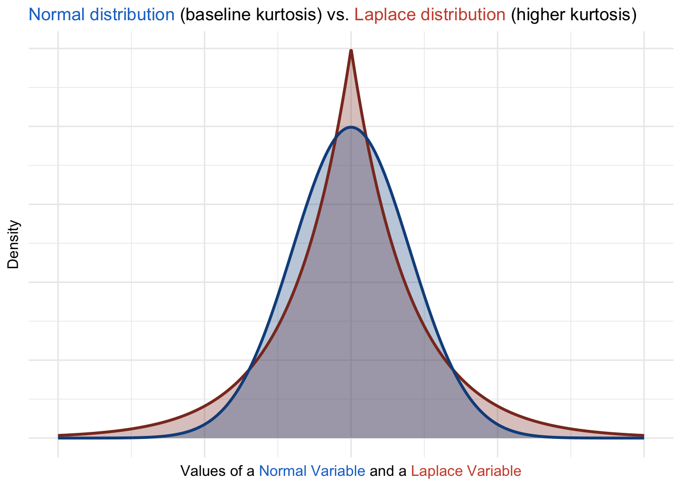
Kurtosis: The Fourth Moment

Kurtosis measures the “tailedness” of a distribution, providing insight into the frequency and magnitude of extreme values. A distribution with high kurtosis has heavier tails and a sharper peak, indicating more frequent extreme deviations from the mean, while low kurtosis reflects lighter tails and a flatter peak. For example, normal distributions have a kurtosis value of 3, which serves as a baseline for comparison.

Entrepreneurial Insights from Kurtosis

Customer Behavior:
- High kurtosis in spending habits might highlight extreme variability among customers, such as a small group of high spenders that significantly impact revenue. Entrepreneurs can target these outliers with premium services or loyalty programs.
- Low kurtosis suggests more consistent spending patterns, making it easier to predict overall revenue and standardize marketing efforts.
Product Feedback and Satisfaction:
- High kurtosis in customer satisfaction scores may indicate polarization, where customers either love or hate a product. This signals the need to investigate underlying causes and either address dissatisfaction or double down on what high-scoring customers value. For example, polarized reviews might guide adjustments in product design, pricing, or marketing strategies to address extreme opinions.
Revenue Stream Analysis: Entrepreneurs can evaluate kurtosis in revenue distributions to assess volatility.
- High kurtosis could signal reliance on irregular, extreme revenue events (e.g., seasonal spikes or a few high-value customers), necessitating risk mitigation strategies such as diversifying revenue streams.
- Low kurtosis might indicate more stable revenue patterns, reducing the need for aggressive risk management.

Demographic Insights: By evaluating kurtosis across demographic groups, businesses can detect differences in variability.
- High kurtosis in spending habits among young customers might suggest diverse financial capabilities, requiring segmentation into premium and budget-conscious categories.
- Low kurtosis within a group may indicate homogeneity, simplifying targeted marketing and product offerings.
Risk and Investment Decisions:
- High kurtosis in metrics like customer lifetime value or project ROI could highlight potential risks, such as over-reliance on outliers for profitability. Entrepreneurs can use this insight to avoid overestimating average performance due to extreme values.
- Low kurtosis indicates a more predictable range of outcomes, which might encourage higher confidence in scaling efforts.

Figure 23.5: Comparison of kurtosis in the standard normal distribution to the higher kurtosis of a Laplace distribution

23.6 Conclusion

Understanding variables and distributions is foundational for any data analysis. Variables capture the core elements of your data, while distributions reveal how their values are clustered and spread. Skewness and kurtosis describe the shape of a variable’s distribution, providing insight into asymmetry (skewness) and the presence of heavy tails or peakedness (kurtosis). These concepts are foundational to understanding how data deviates from a normal distribution as explored in Chapter 25 and exploratory data analysis as explored in Chapter 27.

By learning to identify and interpret measures of central tendency, spread, skewness and kurtosis, you’ve gained essential tools for summarizing data. In the next chapter, we’ll explore how to use confidence intervals and hypothesis testing to draw inferences and make data-driven decisions.