The first step in any data analysis project is to inspect and understand the data. This process allows you to familiarize yourself with the dataset, identify potential issues, and ensure that it is in a state that can be worked with. It ensures that your dataset is clean, consistent, and ready for deeper analysis.
This chapter guides you through the essential tasks of inspecting your data, from understanding its structure and summary statistics to identifying missing values, duplicates, and outliers. Each section provides a focused look at one part of the inspection workflow, helping you systematically assess and prepare your data for analysis. We’ll simplify work by using the janitor package and combine it with a few select functions from base R and tidyverse for deeper understanding.
Let’s practice with a dataset of entrepreneurs named entrepreneur_data that has already been imported into R (and this document).
entrepreneur_data
# A tibble: 10 × 7
   name      age gender sector  revenue_million funding_million years_experience
   <chr>   <dbl> <fct>  <chr>             <dbl>           <dbl>            <int>
 1 Alice      34 Female Tech                1.2             3.5               10
 2 Bob        42 Male   Finance             2.3             1                 15
 3 Charlie    29 Male   Tech                0.9             0.5                5
 4 Diana      NA Female Health              1.8             2                 12
 5 Eve        25 Female Tech               NA               1.8                2
 6 Frank      37 Male   Health              1.1            NA                  8
 7 Alice      34 Female Tech                1.2             3.5               10
 8 Gina       31 Female Finance             2.4             1.1                7
 9 Hank       48 Male   Health              3               2.8               20
10 <NA>       29 Male   Tech               NA               0.5                5
The variables include:
name: Name of the entrepreneur
age: Age of the entrepreneur
gender: Gender of the entrepreneur
sector: The industry sector of the startup
revenue_million: The revenue of the startup in millions
funding_million: The amount of funding received in millions
years_experience: Years of experience the entrepreneur has
16.2 Getting to Know your Data
To begin, let’s get an overall sense of the dataset using the adorn_totals() function from the janitor library and glimpse() function from the dplyr package in tidyverse. The janitor library offers some simple and useful functions for inspecting data that are not found in glimpse().
With adorn_totals() from janitor
adorn_totals() provides the sum (Total) of every variable (column) of the dataset:
## load the janitor library for access to the adorn_total functionlibrary(janitor)## adorn_totals to calculate the totals of each variableadorn_totals(entrepreneur_data)
    name age gender  sector revenue_million funding_million years_experience
   Alice  34 Female    Tech             1.2             3.5               10
     Bob  42   Male Finance             2.3             1.0               15
 Charlie  29   Male    Tech             0.9             0.5                5
   Diana  NA Female  Health             1.8             2.0               12
     Eve  25 Female    Tech              NA             1.8                2
   Frank  37   Male  Health             1.1              NA                8
   Alice  34 Female    Tech             1.2             3.5               10
    Gina  31 Female Finance             2.4             1.1                7
    Hank  48   Male  Health             3.0             2.8               20
    <NA>  29   Male    Tech              NA             0.5                5
   Total 309      -       -            13.9            16.7               94
With glimpse() from tidyverse
glimpse() provides a transposed view of your data with variables listed as rows:
This shows us the structure of the data with variable names, types, and some of the values in each column.1
16.3 Examining Specific Rows
Use the following functions to quickly view specific rows:
With head() and tail()
These functions allow us to see the first and last rows of the dataset, respectively.
head(entrepreneur_data, 3) ## Show first 3 rows
# A tibble: 3 × 7
  name      age gender sector  revenue_million funding_million years_experience
  <chr>   <dbl> <fct>  <chr>             <dbl>           <dbl>            <int>
1 Alice      34 Female Tech                1.2             3.5               10
2 Bob        42 Male   Finance             2.3             1                 15
3 Charlie    29 Male   Tech                0.9             0.5                5
tail(entrepreneur_data, 2) ## Show last 2 rows
# A tibble: 2 × 7
  name    age gender sector revenue_million funding_million years_experience
  <chr> <dbl> <fct>  <chr>            <dbl>           <dbl>            <int>
1 Hank     48 Male   Health               3             2.8               20
2 <NA>     29 Male   Tech                NA             0.5                5
Note
By default, head() shows the first 6 rows, but you can adjust this by specifying the number of rows you’d like to see.
Try it yourself:
Change the code to display the first 7 rows of entrepreneur_data.
Hint 1
head() shows 6 rows by default. Consider what argument you can add to vary from the default number of rows.
Hint 2
Add the desired number of rows (7) as an argument to the function.
head(entrepreneur_data, 3)
Fully worked solution:
Add the desired number of rows to the function as an argument in addition to the tibble name.
head(entrepreneur_data, 3)
Now change the code to display the last 4 rows of the dataset.
Hint 1
tail()) shows 6 rows by default. Consider what argument you can add to vary from the default number of rows.
Hint 2
Add the desired number of rows (4) as an argument to the function.
tail(entrepreneur_data, 4)
Fully worked solution:
Add the desired number of rows to the function as an argument in addition to the tibble name.
tail(entrepreneur_data, 4)
16.4 Understanding Data Structure and Summary Statistics
Data Dimensions
dim(): Returns the number of rows and columns in the data.
nrow() and ncol(): Return the number of rows or columns separately.
dim(entrepreneur_data) ## shows that there are 10 rows and 7 columns
[1] 10 7
nrow(entrepreneur_data) ## shows that there are 10 rows
[1] 10
ncol(entrepreneur_data) ## shows that there are 7 columns
[1] 7
Summary of Columns
summary() provides a quick overview of each column, showing descriptive statistics for numeric variables and frequencies for categorical variables.
summary(entrepreneur_data) ## summarizes every variable
     name                age           gender     sector
 Length:10          Min.   :25.00   Female:5   Length:10
 Class :character   1st Qu.:29.00   Male  :5   Class :character
 Mode  :character   Median :34.00              Mode  :character
                    Mean   :34.33
                    3rd Qu.:37.00
                    Max.   :48.00
                    NA's   :1
 revenue_million funding_million years_experience
 Min.   :0.900   Min.   :0.500   Min.   : 2.0
 1st Qu.:1.175   1st Qu.:1.000   1st Qu.: 5.5
 Median :1.500   Median :1.800   Median : 9.0
 Mean   :1.738   Mean   :1.856   Mean   : 9.4
 3rd Qu.:2.325   3rd Qu.:2.800   3rd Qu.:11.5
 Max.   :3.000   Max.   :3.500   Max.   :20.0
 NA's   :2       NA's   :1
Note
This function is great for spotting potential outliers or missing values.
16.5 Inspecting Data Types and Values
Understanding the types of variables you’re working with is essential:
Structure of the Dataset
Use str() to check the structure of the dataset.
str(entrepreneur_data) ## shows the data type of every variable
Looking closely, we can also see an indicator between the name of the variable and its values. This is an indicator of the data type:
name indicates a character variable meaning that the values of the name variable are made of characters (letters rather than numbers).
age indicates numeric data and, more specifically, double-precision data (numbers that can have decimals).
gender is a category variable which is known as a factor in R.
sector is a character variable for the startup’s industry sector.2
revenue_million indicates double-precision numeric data representing revenue in units of million dollars.
funding_million is double-precision numeric data representing funding in units of million dollars.
years_experience indicates numeric data in integer form (numbers can only be whole numbers).
Checking Types for Specific Variables
You can also check the data type of specific variables with typeof():
typeof(entrepreneur_data$name) ## shows that "name" is character data
[1] "character"
typeof(entrepreneur_data$age) ## shows that "age" is a numeric (double precision) variable
[1] "double"
If you find incorrect data types (e.g., dates stored as strings, numerical values stored as characters), this inspection identifies which variables need to be transformed.
16.6 Identifying Missing Values
Missing data can affect your analysis so let’s check for missing values.
Check for Missing Values with is.na()
is.na(): detects missing values in the dataset.
sum(is.na(entrepreneur_data)) ## Total missing values
[1] 5
colSums(is.na(entrepreneur_data)) ## Missing values per column
            name              age           gender           sector
               1                1                0                0
 revenue_million  funding_million years_experience
               2                1                0
Check for Missing Values with tabyl()
You can also use tabyl() from the janitor library to get a cleaner breakdown of missing values for a specific variable.
## load the janitor librarylibrary(janitor)## get a summary of gender from tabyl()entrepreneur_data |>tabyl(gender, show_na =TRUE)
 gender n percent
 Female 5     0.5
   Male 5     0.5
## get a summary of gender and sector from tabyl()entrepreneur_data |>tabyl(gender, sector, show_na =TRUE)
 gender Finance Health Tech
 Female       1      1    3
   Male       1      2    2
Check for missing values with skim()
skim() (from the skimr package): Provides a more detailed overview of missing values along with summary statistics.
library(skimr) ## load the libraryskim(entrepreneur_data) ##
Data summary
Name
entrepreneur_data
Number of rows
10
Number of columns
7
_______________________
Column type frequency:
character
2
factor
1
numeric
4
________________________
Group variables
None
Variable type: character
skim_variable
n_missing
complete_rate
min
max
empty
n_unique
whitespace
name
1
0.9
3
7
0
8
0
sector
0
1.0
4
7
0
3
0
Variable type: factor
skim_variable
n_missing
complete_rate
ordered
n_unique
top_counts
gender
0
1
FALSE
2
Fem: 5, Mal: 5
Variable type: numeric
skim_variable
n_missing
complete_rate
mean
sd
p0
p25
p50
p75
p100
hist
age
1
0.9
34.33
7.14
25.0
29.00
34.0
37.00
48.0
▇▇▂▂▂
revenue_million
2
0.8
1.74
0.76
0.9
1.17
1.5
2.32
3.0
▇▁▂▃▂
funding_million
1
0.9
1.86
1.19
0.5
1.00
1.8
2.80
3.5
▇▁▃▂▃
years_experience
0
1.0
9.40
5.30
2.0
5.50
9.0
11.50
20.0
▇▅▇▂▂
The only thing we know for sure about a missing data point is that it is not there, and there is nothing that the magic of statistics can do do change that. The best that can be managed is to estimate the extent to which missing data have influenced the inferences we wish to draw.
– Howard Wainer
16.7 Checking for Duplicate Records
Duplicate data can skew your analysis. Use janitor to find duplicates.
Identify and Remove Duplicates
library(janitor) ## load the libraryentrepreneur_data |>get_dupes()
# A tibble: 2 × 8
  name    age gender sector revenue_million funding_million years_experience
  <chr> <dbl> <fct>  <chr>            <dbl>           <dbl>            <int>
1 Alice    34 Female Tech               1.2             3.5               10
2 Alice    34 Female Tech               1.2             3.5               10
# ℹ 1 more variable: dupe_count <int>
This finds rows that have duplicate values across all columns.
16.8 Detecting Outliers
It’s not uncommon for datasets to contain errors that result in extreme or unexpected values. These issues can arise from various sources, such as:
Data entry errors: Typographical mistakes, such as misplaced decimal points, leading to values that are much too large or too small.
Formatting inconsistencies: Numbers stored with thousands separators (100,000) or abbreviated as character strings (100K) instead of raw numbers (100000).
Sign errors: Positive values entered as negative (or vice versa).
Survey anomalies: Respondents providing extreme or nonsensical values, sometimes intentionally.
Identifying these extreme values, often called outliers, is a crucial part of data inspection. Outliers can significantly distort your analysis if left unaddressed, so it’s essential to investigate their cause.
Dealing with Outliers
When outliers are identified, the next step is to decide how to handle them. Here are some guiding principles:
Fix known errors: If an extreme value is the result of a known data entry or formatting error, and you can confidently correct it, do so.
For example, in historical data from the production of Liberty Ships during World War II,3 one ship appeared as an extreme outlier in production time and cost. Curious about this anomaly, I returned to the original government data files and referenced a book by a program manager from that era. Through this research, I discovered that the ship had been used as target practice for Navy bombers, not for actual production. Confident in the reason behind the anomaly, I removed this ship from the dataset to prevent it from skewing the analysis.
This example highlights the value of persistence and curiosity when investigating outliers. As an analyst, you should be prepared to dig deeper, returning to source materials or consulting domain experts, to understand the true nature of your data.
Remove clearly invalid values: Outliers that are demonstrably wrong, such as a temperature reading of 1,000 degrees in a dataset about human body temperatures, should be removed.
Exercise caution with unknowns: Be hesitant to remove or manipulate data simply because it’s surprising. Outliers might represent valid, unexpected phenomena or new insights. Removing such values without thorough investigation risks introducing bias and missing opportunities to learn from the data.
The first step is to find the outliers:
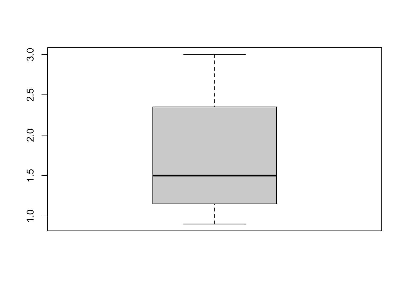
Visualizing Outliers
Use a simple boxplot to spot outliers.
boxplot(entrepreneur_data$revenue_million)
Counting Categorical Frequencies
Use tabyl() from the janitor library can also summarize categorical data frequencies.
library(janitor) ## load the libraryentrepreneur_data |>tabyl(sector) ## use tabyl to check for outliers in sector
  sector n percent
 Finance 2     0.2
  Health 3     0.3
    Tech 5     0.5
This shows a breakdown of the counts in the sector column.
Checking Maximum and Minimum Values
As mentioned earlier, summary() from base R provides a quick way to identify outliers in numeric columns by showing the minimum, maximum, and quartiles.
entrepreneur_data |>summary() ## use summary() to check for outliers
     name                age           gender     sector
 Length:10          Min.   :25.00   Female:5   Length:10
 Class :character   1st Qu.:29.00   Male  :5   Class :character
 Mode  :character   Median :34.00              Mode  :character
                    Mean   :34.33
                    3rd Qu.:37.00
                    Max.   :48.00
                    NA's   :1
 revenue_million funding_million years_experience
 Min.   :0.900   Min.   :0.500   Min.   : 2.0
 1st Qu.:1.175   1st Qu.:1.000   1st Qu.: 5.5
 Median :1.500   Median :1.800   Median : 9.0
 Mean   :1.738   Mean   :1.856   Mean   : 9.4
 3rd Qu.:2.325   3rd Qu.:2.800   3rd Qu.:11.5
 Max.   :3.000   Max.   :3.500   Max.   :20.0
 NA's   :2       NA's   :1
16.9 Conclusion
Inspecting and understanding your data is an essential first step in the data analytics process. By getting familiar with the structure, identifying issues like missing values or incorrect data types, you set yourself up for success in the data cleaning and transformation stages.
In this small dataset with only 10 rows, adorn_totals and glimpse() are both able to show all of the data. For larger datasets, they show a subset of the first several values of each row.↩︎
sector is probably better classified as a factor type. We will learn how to convert it from character to factor in Section 21.4.↩︎
See Section 18.2 for more details about the production data of Liberty Ships.↩︎